The point data tables (head, efficiency or power, NPSHr, & submergence) capture the individual data points for the diameters, speeds, widths or pitches specified in the impeller diameter table. Performance curves will be generated from the point data provided. The "generated" performance curves (not the actual data) will be used by the Selector. Options to improve the fit between the generated curve and the actual point values are provided to help produce the best possible curve output results. These options include: disabled, on-curve, slope=0, division point, and slope continuity at division point. See below to learn how to populate and manipulate the data point tables.
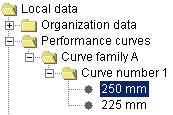
In the navigational tree, open the performance curve folder, curve family folder, curve number folder, and select the impeller diameter for which the point data is to be populated.

*This example shows the 250 mm diameter selected.
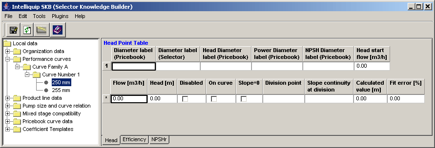
The data manager pane will default to display the head point table. Four taps located at the bottom of the pane (Head, Efficiency or Power, NPSHr, and Submergence) correspond directly to the each of the point data tables. Select a tab to display the appropriate point data table. (The head tab is selected by default when first entering the point data table section). Click here to see an example.

Information from the impeller table will be displayed at the top of each point data table. These fields are active and can be updated or edited as appropriate.
Enter the appropriate data in the first row identified by the asterisk.
Press Enter to accept the data. ( The asterisk will change to a 1).
Use the append function to insert more rows and enter the remaining data points necessary to represent the curve. If desired, point data can be copied from excel and pasted into the tables.
Important
 :
A minimum of five (5) data points are required to generate a curve.
Click to save the data.
To populate the remaining tables, select the appropriate table and repeat steps 3 through 6.
From the data points entered, the SKB will generated curves based on a 4th order polynomial. This method in most cases will be sufficient in producing the expected output curve which the Selector will use. However in cases when the generated curve ( the curve produced for the calculated values) does not represent or meet the expectations of the entered data, it may become necessary to "adjust" the curve to produce a better representation of the expect output. Four options are provided to make adjustments, these include: disabled, on-curve, slope=0, division point, and slope continuity at division.
In each data point table, the calculated value column displays the values which are used to generate the performance curves used by the Selector. The percent deviation between the actual and calculated values are shown in the fit error column field. If the percent deviation exceeds the fit error limit value set in the curve family table the cells background will become red to indicate that it may be necessary to adjust the generate curve to improve the "fit". The options below are provided to make the adjustments.
Note: Multiple options can be selected in each data point table. It is also good practice to view the curve after selecting each option.
Disabled - Selecting this option will disable the data point from the graph. A data point that has been disabled will be shown in red on the curve graph.
On curve - This selection will force the curve through the data point. A good use for this option would be to force the curve through the BEP point to ensure maximum efficiency is reached.
Slope=0 - This option will force the curve's slope to equal zero at that particular point.
Division point - When a division point is specified, the SKB will generate separate curves joined at the division point. For this option to be available there must be a minimum of nine data points.
Slope continuity at division - When enabling this option, the SKB will maintain the slope of the generated curve through the division point. When disabling this option, the SKB will generate two separate slopes for the curves joined at the division point.
Click
this image to see an example of a data point table with curve options
applied. 